
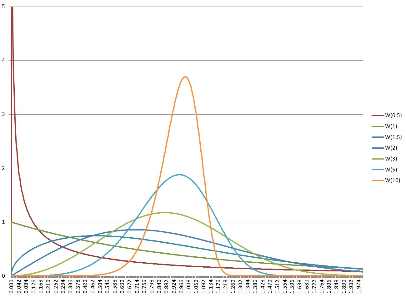
Weibull distribution shapes depend on the shape parameter
In my previous post, I referred to the insight (created by experts who have analyzed lots of real-world software and IT project data) that lead times in such projects often have the Weibull distribution. I also explained a bit what this distribution is and showed a method to quickly test whether your data set matches this distribution and it it does what is it’s shape parameter. Remember, Weibull is a parametrized family of distributions, each distribution is identified by the shape parameter, which tweaks the shape of the distribution curve. This parameter is characteristic of how the work tends to expand and get interrupted in a particular context, so it characterizes the system of work where the project is being carried out.
Now I’d like to identify some practically useful properties of this distribution. Most of them are linked to the shape parameter, denoted by letter k, so it is very important to know what this parameter is in your context. I also want to limit the scope to shape parameter range between 1 and 2, because, as I learned from Troy Magennis, k=1.5 is fairly common in software/IT projects.
Forget the Three Sigmas
Calculating the standard deviation for this distribution is meaningless. The mean and the standard deviation are often thought of as two separate variables characterizing a distribution, and the following may be counter-intuitive to those who are used to Gaussian bell curves, but the Weibull distribution’s nature is that its standard deviation and mean are linked strictly. Not only that, but all the numbers we need from the distribution are also proportional to the mean and the proportion depends only on the shape parameter. What are these numbers that we care about?
- The median – what’s the over-under of how long this work will take? Because Weibull is asymmetric, this is not equal to the mean.
- The mode. When we think about estimating work, our brains may be primed for the most often-occurring numbers. But as we will soon see, the most often-occurring number may be quite far and on both sides of the mean and the median.
- Important percentiles, such as 80%, 95% – what is the timeline for completing the work with such probability?
- The statistical process control limits – the equivalents of plus-minus-three-sigma for normal distributions.
- The ratio of the mode to the upper control limit – practitioners of Product Sashimi can probably guess why.
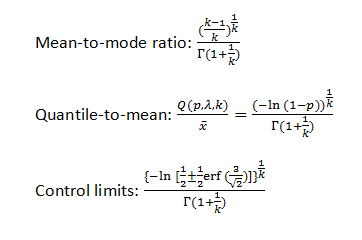
Here are all the necessary formulas:
Results
Here are the results. To keep the table compact, the mode, the median and the percentiles are expressed as their ratios to the mean. I also dropped the lower control limits from the table, because they are all very close to zero.
| k | Mode | Median | 80% | 95% | UCL | Mode/UCL |
| 1.1 | 0.117 | 0.743 | 1.487 | 2.616 | 5.768 | 2.0% |
| 1.2 | 0.239 | 0.783 | 1.398 | 2.437 | 5.128 | 4.7% |
| 1.3 | 0.350 | 0.817 | 1.332 | 2.148 | 4.627 | 7.6% |
| 1.4 | 0.448 | 0.844 | 1.280 | 1.996 | 4.227 | 10.6% |
| 1.5 | 0.533 | 0.868 | 1.240 | 1.876 | 3.901 | 13.7% |
| 1.6 | 0.604 | 0.887 | 1.207 | 1.780 | 3.630 | 16.6% |
| 1.7 | 0.665 | 0.903 | 1.180 | 1.701 | 3.403 | 19.5% |
| 1.8 | 0.717 | 0.917 | 1.158 | 1.636 | 3.210 | 22.3% |
| 1.9 | 0.761 | 0.929 | 1.140 | 1.581 | 3.044 | 25.0% |
| 2.0 | 0.798 | 0.939 | 1.124 | 1.534 | 2.901 | 27.5% |
What can we see here? The most-frequently occurring lead time — which may stick in our memory and which we as estimators may be biased towards — may be as little as 20-40% of the mean. At the same time, the timeline 80% delivery guarantee can be 40% longer than the mean. Providing delivery guarantees beyond 80% is very expensive. The Weibull tail is significantly fatter than the normal distribution’s tails.
The ratio of mode to the upper control limit can be useful to teams using iterative development methods. It shows how the time to complete a typical user story (from selecting it during sprint planning to meeting the definition of done) relates to the iteration length. It confirms what XP practitioners knew all along: keep them much smaller than the iteration length.
For the popular shape parameter value 1.5, the ratio of the upper control limit to the mean is approximately 4. This can be used as a rule of thumb to estimate one of these numbers after observing the other.


Where the formulas come from? I was not able to find any literature that supports them.
Dimitar, thank you for the comment. The formulas are from http://en.wikipedia.org/wiki/Weibull_distribution
I rechecked my math. The formula for the quantile, which is important for calculating the median, the 80% and 95% percentiles and the control limits is Q(p,x,lambda) = lambda*(-ln(1-p))^(1/k). The mean is lambda*gamma(1+1/k), so in the quantile-to-mean ratio, the scale parameters lambdas cancel each other out, producing the formula (2) above.
Formula (3) is the same as formula (2), where I substituted the p-th quantile with the 1/2+-1/2*erf(3/sqrt(2)), which is a pair of constants that equal the quantiles corresponding to plus-minus three standard deviations on the normal distribution. These two formulas should be correct.
In formula (1), I made a mistake, dropping the denominator as I tried to draw the formula. Thank you for catching it. The denominator should contain gamma(1+1/k), so the whole formula for the mode-to-mean ratio is ((k-1)/k)^(1/k)/gamma(1+1/k).
I’m going to update the numbers in the mode-to-mean and mode-to-UCL columns, but they won’t change significantly, because gamma(1+1/k) is close enough to unity. The reasoning in the next-to-last paragraph about how the time to complete a user story in an iterative process relates to the iteration length is still valid.
this is actually pretty amazing stuff, thanks for that!
I myself kind of accidentally stumbled upon this whole “Weibull-topic” and now I’m totally hooked by it as more and more things get clearer each time I see our distributions from this unique new perspective… I’ve read the paper by Troy Magennis and of course all of your stuff but I’m somewhat stuck with the above table… could you please try to elaborate on it once more? What are the direct implications I might be able to deduct from it when dealing with real data from my IT department? I somehow missed out on the bridge… THANKS
Nils, thank you for finding this post. It’s from old times, though, when there was a thing I’d now described as “the Weibull crutch.” It was an intellectual crutch that helped me and several others understand the nature of variation on knowledge work. The Weibull shape parameter can give Weibull distribution very different qualities. With k2, you get very thin tails, like Gaussian or even thinner. With 1<k<2, you get something in the middle. As we understand it today, the actual distributions of time in knowledge work may or may not follow Weibull, but they fall into these three broad classes. And the Weibull k=1 (also known as Exponential) and Weibull k=2 (also known as Rayleigh) distributions are useful to demarcate the boundaries between them. The practical interpretation of the three classes is as follows. 1) Very thin tails — if time in your knowledge work looks like this, what you do is a target for automation and disruption, very fragile. 2) Fat tails — you've got a fragile process, loaded with risks of delay such as dependencies, blockage, queues, and preemption. 3) In the middle, you've got well-managed knowledge work.